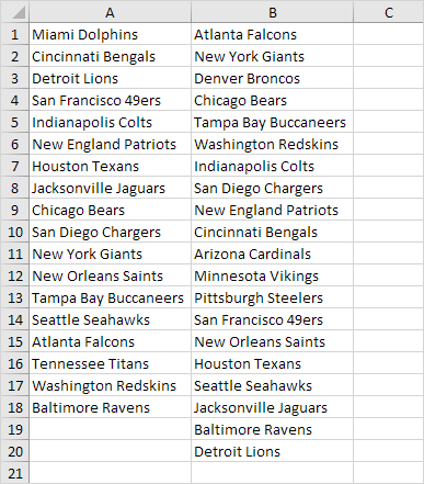
1. Select the range A1:A18 and name it firstList, select the range B1:B20 and name it secondList.

2. Select the range A1:A18
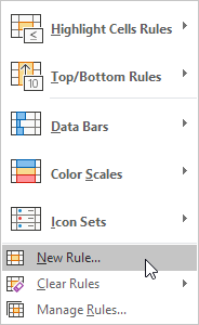
3. On the Home tab, click Conditional Formatting, New Rule...
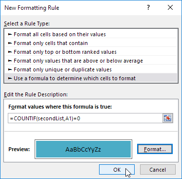
4. Select "Use a formula to determine which cells to format".
5. Enter the formula =COUNTIF(secondList,A1)=0
6. Select a formatting style and click OK.
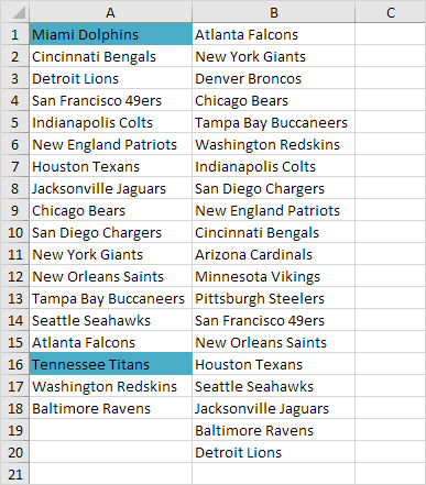
7. As a result, Miami Dolphins and Tennessee Titans are not in the second list.
Note: =COUNTIF(secondList,A1) counts the number of teams in secondList that are equal to the team in cell A1. If COUNTIF(secondList,A1) = 0, the team in cell A1 is not in the second list. As a result, Excel fills the cell with a blue background color. Because we selected the range A1:A18 before we clicked on Conditional Formatting, Excel automatically copies the formula to the other cells. Thus, cell A2 contains the formula =COUNTIF(secondList,A2)=0, cell A3 =COUNTIF(secondList,A3)=0, etc.
8. To highlight the teams in the second list that are not in the first list, select the range B1:B20, create a new rule using the formula =COUNTIF(firstList,B1)=0, and set the format to orange fill.
9. As a result, Denver Broncos, Arizona Cardinals, Minnesota Vikings and Pittsburgh Steelers are not in the first list.

Reference:
Compare Two Lists
http://www.excel-easy.com/examples/compare-two-lists.html
No comments:
Post a Comment